Learning Rules

Quickprop [fahlman88empirical]

Equation 1. Error derivative at previous epoch

Equation 2. Error derivative at this epoch

The Quickprop algorithm is loosely based on Newton's method. It is quicker than standard backpropagation because it uses an approximation to the error curve, and second order derivative information which allow a quicker evaluation. Training is similar to backprop except for a copy of (eq. 1) the error derivative at a previous epoch. This, and the current error derivative (eq. 2), are used to minimise an approximation to this error curve. The update rule is given in equation 3:

Equation 3. Quickprop update rule

This equation uses no learning rate. If the slope of the error curve is less than that of the previous one, then the weight will change in the same direction (positive or negative). However, there needs to be some controls to prevent the weights from growing too large.

RProp (Resilient Propagation) [riedmiller93direct]

RProp uses a technique that differs from backpropagation by the weight update which is done without using the gradient information. or a learning rate parameter. A quantity, called the update value, is added to the weight at each iteration. Its value and sign are governed by the gradient sign technique, such that the error function is minimised:

Equation 4. RProp Updating

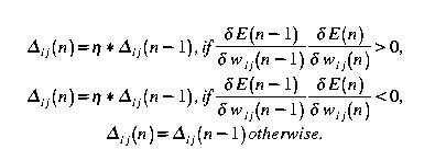
RProp is a batch updating algorithm. It is very fast. The weight updating algorithm is expressed in figure 5:

Quickprop and RProp are both algorithms for feedforward neural networks, and both will require the FeedforwardArchitecture class. As far as implementation is concerned, both of these could inherit BackpropagationLearningRule as the theories themselves derive from backpropagation so apart from the weight updating methods which differ, the implementation remains the same.

Cascade Correlation [fahlman91cascadecorrelation]

The cascade correlation algorithm constructs an ANN by adding hidden units one by one. There are two training stages: (1) maximising correlation between the network residual error and the newly added hidden neuron's output (learning the weights from input to hidden layers); (2) minimising network error while freezing all weights to the hidden node (from the hidden to output layers).

The correlation (covariance) is defined as the function in eq. 6:

Equation 5. Correlation (covariance)

Cascade correlation uses another learning rule, such as backpropagation or its variants in conjunction with adding neurons.

Optimal Brain Damage (OBD) [lecun90optimal]

OBD is the name given to the technique of removing unimportant weights during network training (often called pruning). OBD can be applied in particular to those networks previously discussed. Networks that used pruning have been found to have better generalisation, require less training patterns and have better/faster overall performance.

OBD is a technique that selectively deletes weights from a trained neural network, reducing the network size. This works because it reduces the dimensionality of the network. OBD is viewed as a minimisation procedure. Essentially, take a good network, remove half of the weights and end up with a network that works just as well (no reduction in generalisation ability) or better (quicker, reducing network complexity).

OBD can be expressed as follows:

1. Choose a network; architecture

2. Train the network;

3. Compute the second derivatives of the Hessian weight matrix for each parameter;

4. Compute the saliencies for each parameter;

5. Sort the parameters by saliency and remove the lowest salient parameters

6. return to stage 2.

The saliencies are parameters which represent the efficacy of individual connections. It is defined as the change in the objective function if the connection were to be removed

As mentioned before, the OpenAI classes don't currently include a facility for adding or removing network connections, so the architecture class needs to allow for this, either by adding a method to the abstract base class or including it in a derived class.

Radial Basis Function Networks [orr96rbf]

RBFNs are two layer feedforward networks. Network training is divided into two stages: The first determines weights from the input to hidden nodes. These weights represent the centres of radial basis functions. A radial basis function is a function for each data point, of the form in equation 6:

Equation 6. Radial Basis Function

RBFN networks do not have anything that is the same as the bias term present in the MLP.

There are many techniques that are involved with RBFNs, and the an implementation will have to consider all of them. For example, the choice of radial basis function, fixed centres selected at random or normalised RB functions.

It is not necessary to go into depth into the stage two algorithms, it is enough to say that they are straightfoward linear, supervised algorithms.

Problems which are applicable to MLPs are also applicable to RBFNs. The roots of RBFNs are in Cover's theorem and universal function approximation, and its mathematical foundation is very strong. This has made the RBFN a popular choice of network.

Genetic Learning Rule G-Prop [castillo99gprop]

G-prop uses a combined genetic algorithm GA and backpropagation approach for network training. the GA selects the initial set of weights and number of hidden units by applying genetic operators. The theory goes that a global GA search is combined with a local BP search for a more effective training procedure.

GAs can be applied to neural network learning in several ways (for a comprehensive review of evolutionary methods with neural networks see [yao_ie3_proc_online]):

• Searching for an optimal set of weights

• Search over topology space

• Search for optimal learning parameters

• Genetic approach to modify a training algorithm, such as BP

The full G-Prop algorithm is as follows:

• Generate an initial population with random weights and a random number of hidden units within a defined range (from 2 to MAXHIDDEN)

• Repeat for G generations

  1. Evaluate the individuals of the population - train them and assign a fitness value based on their error and/or number of training epochs

  2. Select the N fittest individuals and apply a mating or crossover function. Doing this guarantees diversity.

  3. Replace the unfit individuals with new ones

• Use the best individuals to obtain the testing error

The speed of a GProp network can be inhibitive, but is an interesting method, especially considering its combined application with the OpenAI genetic algorithm classes.

Time Delay Neural Networks (TDNNs)

The TDNN is a specific kind of neural network, discussed here for its obvious practical implications and its relative simplicity. A TDNN is essentially the same as an MLP except with a single feedback connection from the single output neuron to the input (see figure 2). An input is given as f(t - n) ... f(t), where f is an arbitrary time series problem for which the value f(t + 1) is needed. n is the number of inputs. The network is used to predict f(t + 1) which is the value of the output node. The next epoch is used to predict f(t + 2) with inputs now f(t _ n + 1) ... f(t + 1), and so on. The feedback connection may or may not have a weight different to unity.

Kohonen Self Organising Maps

This is an unsupervised learning algorithm which maps an input vector to an output array of nodes. A reference vector, w_ji, is assigned to each of these nodes. An input vector, x_i, is compared with it and the best match of all the neurons is the response. This is what is involved in competitive learning. The winner is the neuron with the best response; the neuron where the Euclidean distance between its weight s and the input pattern is the smallest.

Equation 7. Euclidean distance

The next stage is cooperation. A neighbourhood of neurons is defined around the winning neuron. The neurons in this neighbourhood will all have the chance to update their weights, though not as much as the winner, and the size of the update decreases for neurons as they are further away. Neighbourhoods are usually symmetrical.

The neighbourhood can be defined in one of a number of ways, including defining a square around the winning neuron or commonly using a Gaussian function.

Equation 8. Gaussian Function to Define Neighbourhood Size

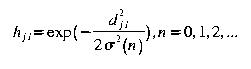
Learning Vector Quantisation (LVQ)

Learning Vector Quantisation is a technique which improves the performance of SOMs for classification. SOM is an unsupervised learning algorithm, but can be used for supervised learning. For example, each neuron of the SOM can be labelled after training. By further supervised learning using LVQ, a two stage learning adaptively is used to solve a classification problem.

The algorithm for SOM learning with LVQ is as follows:

• execute SOM algorithm to obtain learned set of vectors;

• label the neurons;

• LVQ:

• Find the weight that is closest to the input pattern X;

• If the classes of the output neuron vector and the input are the same:

  • Move the neuron vector (weight) closer to the input;

  • Otherwise moving them away from the input (equation).

Equation 9. Learning Vector Quantisation

SOM is used for unsupervised learning, classification and optimisation. Also, returning to the RBFN example, SOM learning can be used for the first (input to hidden layer) stage of learning.